Preamble

SDP is Edinburgh University’s third year Computer Science System Design project. The task is to build and develop a robot to play two-a-side football loosely based on the rules of the RoboCup SSL. Teams have twelve members in two groups of six, one per robot. The System architecture, at an abstract level, is comprised of a vision system, strategy AI/planner, computer-to-robot communications module and of course the robot with it’s hardware and firmware.

Tasks for developing the system were divided up between the ten people in the team, and I took building the code that runs on the Arduino. Provided hardware was the Xino RF, an Arduino clone with the familiar AT328P microcontroller and an added Ciseco SRF chip, for wireless communications to the C&C computer that’d be running the rest of the stack.

Holonomics are fun

Our group settled on a three wheeled holonomic design pretty early on - motivations for this were mainly “Because it’s cool”, “Angus wants to do holonomics” and also because some people in the year above strongly suggested that we didnt’t make a holonomic robot. Holonomic wheels have bearings that let the wheel slide laterally along it’s axis of rotation, giving freedom of movement in any direction if used correctly.

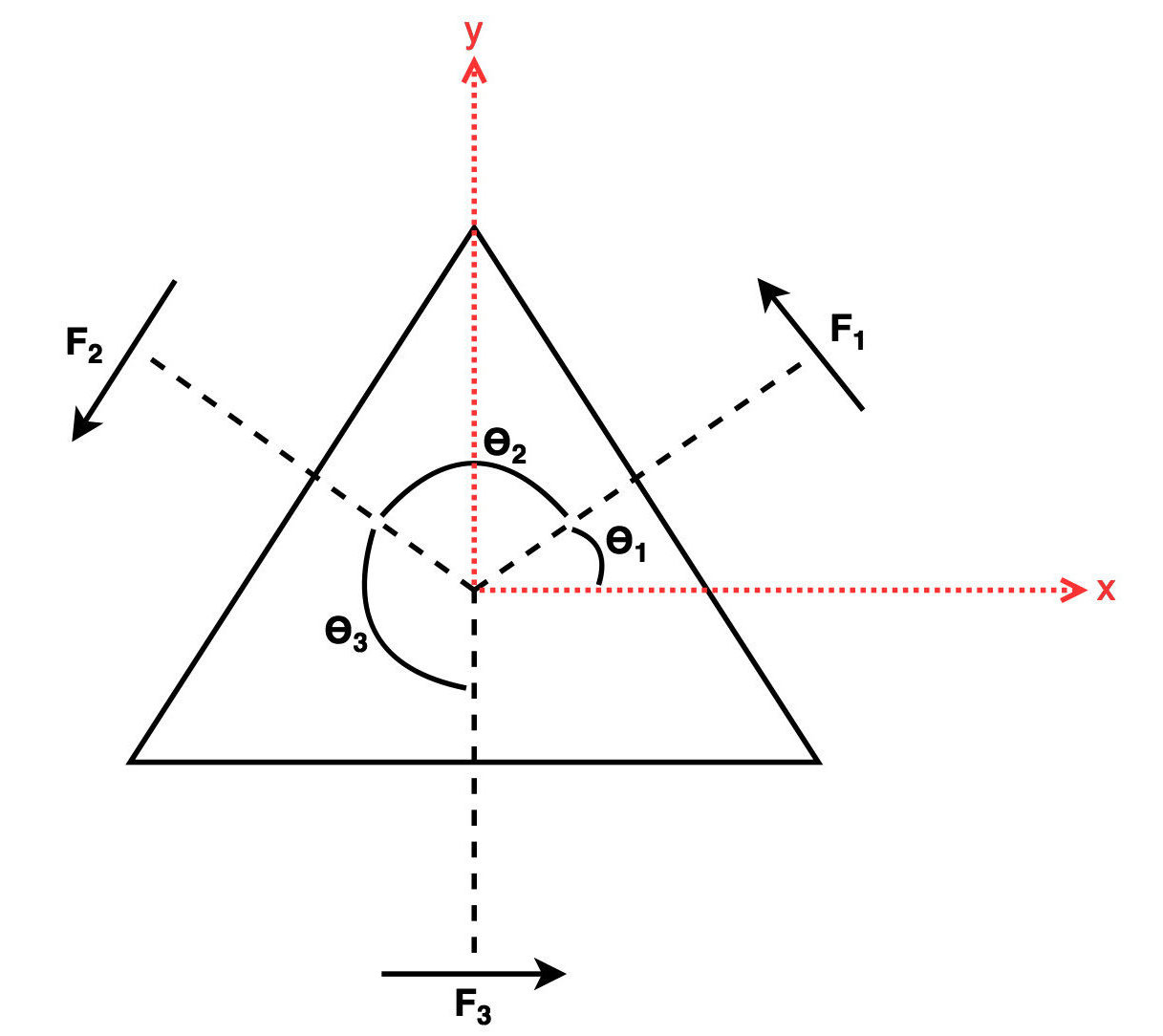
The maths behind holonomic motion isn’t actually all that complex - it comes from doing the mechanics on the three forces produced by the three wheels, and the observation that what we’re really dealing with is a matrix.

Simple trigonometry splits these forces into their x,y components.

So, we have the following:

Which, is equivalent to the following Force Coupling matrix: (Note the omega is the rotational force)

This translation between forward, lateral & rotational force and the application of power is done in firmware, meaning the rest of the stack needn’t be aware of the specifics of this bot; Three wheel holonomic or otherwise. While the single-precision floating point we’re limited to on the Arduino (double is a lie) makes this tricky, in practice using unit vectors and a separate magnitude multipliers prevents NaNs from making everything explode.

Error correcting on the fly

While holonomics are a powerful advantage, giving the ability to move in any direction independently of rotation, this all depends on us being able to move the motors in perfect proportions to the holonomic forces we’ve derived using the above matrix.

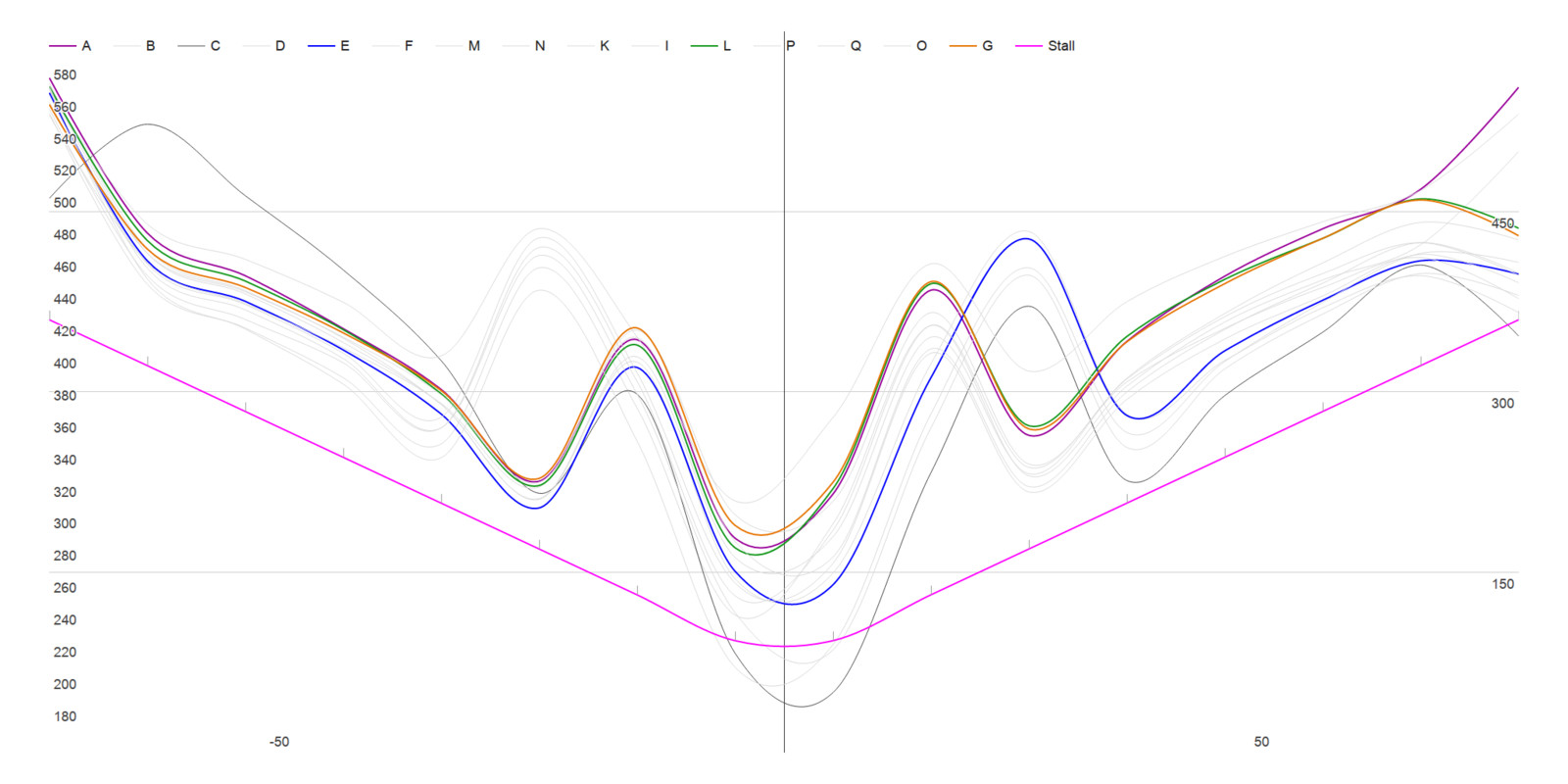
It’s also not sufficient to try correcting linearly, nor is it particularly clever to guess at some function that’ll do this correction for you. The graph below shows the uneven relationship between the rotational speeds of the motors and the applied power.

The motors were run from -100% to 100% power quickly, so this graph only shows how the rotational speeds are unstable, not that the power doesn’t correlate to speed. The three coloured lines that are closely grouped are the three motors selected for use on our bot; The single blue line is a particularly broken motor, and the pink line indicates a stall condition - if the motor is running below this line, we’re probably trying to shove a wall or robot around.

A full PID controller is probably overkill in this situation, so we employed a Gradient Descent algorithm to do these corrections during runtime, using the feedback from the rotary encoders Lego’s NXT motors are equipped with.

So, without further ado, the correction maths on the robot: The error vector \(\hat{e}\) given a desired velocity vector (The one we get sent over the RF link) \(\hat{d}\) and realised velocity vector \(\hat{r}\) (the one we read from the rotary encoders) is:

\(k\) is the learning rate, which varies the granularity with which we’ll correct, hopefully resulting in a smooth correction with no over-reactions. Tuning this constant has the greatest effect on how the corrective system behaves; We used a value of around 0.1, which is quite conservative but very smooth given corrections are being made 20 times a second. This also prevents the robot from confusing a sudden commanded change in direction with a massive error, given the controller isn’t complex enough to model the fact we can’t instantaneously change direction.

The new powers we need to apply to the motors, \(\hat{c'}\) to reduce the error with respect to the previous \(\hat{c}\) and error \(\hat{e}\) is

Note that we’re operating on unit length vectors here - that prevents the need to consider the units we’re working in, some of which would take a large amount of unnecessary computation to figure out. After we’re done correcting, a power multiplier scales the corrected unit vector back up.

So, the error function we need to minimise, \(E\), is as follows: (bit of a maths jump, it’s just the size of \(\hat{e}\))

Finally, for Gradient Descent correction we need the partial derivative of \(E\) with respect to \(\hat{r_i}\)

And the result of all this fiddling looks like this: (Warning: loud NXT motor noise)

Doing more than one thing

It’s pretty important that the bot can perform more than one task at a time - commands could be coming in from strategy, and there’s a host of things we need to do, like reading sensors at steady intervals and performing error corrections.

The code we used in the final round was polling rotary encoders over 20 times a second, sensors that increment a counter every time the wheel went through 1°, then applying the above Gradient Descent correction at the same rate. Coupled with any other tasks the bot was required to execute, a more capable approach to scheduling is needed than just a very large void loop() function.

Our bot used a simple process model, with structures carrying around information about when the task was last run, how often it should be run and whether it was enabled. There were more than eight of these on the bot, which doesn’t seem a lot but given the 16MHz clock speed and limited calculation abilities of the ATMega 328 isn’t a light load.

typedef struct {
    pid_t id;
    unsigned long last_run, interval;
    bool enabled;
    void (*callback)(pid_t);
    const char *label;
} process;

Above, Process structure definition. It’s a tad shorter than the one Linux uses. Below, an example of a process, the one that polls the rotary encoders.

/*
  Rapidly check motor rotations and speeds
*/
const char update_motors_l[] = "update motors";
void update_motors_f(pid_t);
process update_motors = {
    .id         = 0,
    .last_run   = 0,
    .interval   = 50,
    .enabled    = true,
    .callback   = &update_motors_f,
    .label      = update_motors_l
};

A terse yet capable Processes class manages these tasks, which has the advantage of abstracting control logic away from functions that make the robot do something useful, and that once you know the process control logic functions correctly, that any processes that are later added will also be executed as expected.

Processes maintains a list of pointers to these structs, and processes were run in order if last_run + interval is less than millis(). While it is possible to have a runaway condition where no processes runs on time because everything before it is taking too long, that’s essentially the case where you’re tying to do too much on the Arduino.

One of the key functions of processes is that they can be enabled and disabled during runtime, and that the Processes class provides methods for processes to mutate themselves and each-other. This leads to emergent Finite State Machine behaviour, with tasks like grabbing the ball and kicking being done by coding up a set of states and managing transitions between them.

All in all, the result of the synchronous process abstraction and asynchronous command set listening leads to the rather neat main loop() function:

void loop()
{
    CommandSet.readSerial();
    processes.run();
}

Edited 2016-09-14, 2016-12-02, 2017-01-21